D. Rose - March, 2017

---

Abstract

In the world of digital signal processing, the precise value of a signal is known only at specific points. Interpolation is the process of estimating the value of the signal at arbitrary locations between those known points. This paper discusses three different interpolation scenarios: (1) Interpolating a one-dimension signal, such as an audio signal; (2) Interpolating a two-dimensional signal, such as an image; and (3) Interpolating between a series of points on a two-dimensional surface, such as when fitting a smooth curve in a graphics application. The techniques used in this paper are based on the Catmull-Rom cubic spline, which provides a good tradeoff between computational complexity and quality of result.

---

General Solution - Interpolating a One-Dimensional Signal

Figure 1 shows a series of points from a one-dimensional waveform that has been sampled at regular intervals (red dots). Our objective is to approximate the value of the original waveform at some of the unsampled locations between the red dots (show by the blue dashed line).

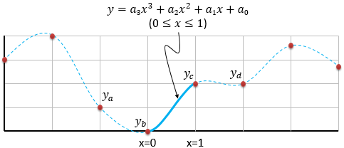
Figure 1: The objective is to find a smooth curve (blue line) that passes through each of the original samples (red dots)

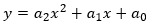
Our approach is to find an equation that describes the continuous waveform for each segment, where a segment is defined as the gap between consecutive samples (for example, the solid blue line in Figure 1). The equation we will use is a cubic polynomial, which has the general form:

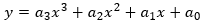
Equation 1 has four unknown coefficients (a₀ through a₃), which can be calculated using the four sample values that surround the segment as follows:

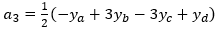
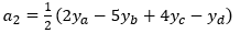
So, given four consecutive samples—y_a, y_b, y_c and y_d—we can compute the four coefficients that define equation 1. Plugging x=0.0 into equation 1 will produce a y value of y_b, and plugging in x=1.0 will produce a y value of y_c. Varying x smoothly between 0.0 and 1.0 will generate the intermediate y values.

We repeat this process for every segment, producing a new set of polynomial coefficients for each. Note that each segment’s polynomial is always evaluated between 0.0 and 1.0, regardless of its position in the overall waveform.

Special Case—Interpolating the End Segments

The astute reader will have noticed that the above solution requires two points to the left and two points to the right of the segment being estimated. How do we find the equation for the very first and very last segments, which are each missing one of the requisite four points? There are several possible solutions, such as assuming the missing point has a value of zero, or replicating the first or last point to use in place of the missing sample. However, both of these can produce non-intuitive results for some combinations of data. A solution we have found to work well is to model the two end segments using a quadratic (a second-order polynomial) instead of a cubic, as illustrated in Figure 2:

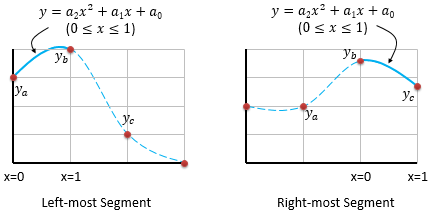
Figure 2: The segments at the left and right ends of a series are modeled using a quadratic. Only three samples are required to solve for the three coefficients.

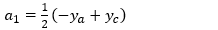
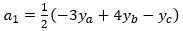
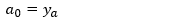
For the left-most segment, the equation for the curve between y_a and y_b has the general form:

Where the coefficients are:

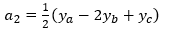
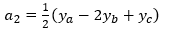
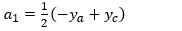
For the right-most segment, the equation for the curve between y_b and y_c has the general form:

Where the coefficients are:

Proof

One can implement the above interpolation technique without knowing how the equations were derived. However, for the curious, the Caltmull-Rom interpolation method is based on the following four constraints (referring to Figure 3):

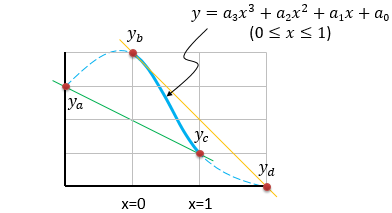
Figure 3: Derivation of the Catmull-Rom Spline equations. The value and slope of the curve is constrained at x=0 and x=1.

1. The curve must pass through y_b
2. The curve must pass through y_c
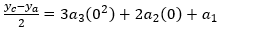
3. The slope of the curve at y_b must equal the slope of a line drawn between y_a and y_c (the green line in Figure 3). That is, the slope at x=0 must equal (y_c - y_a)/2.
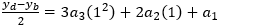
4. The slope of the curve at y_c must equal the slope of a line drawn between y_b and y_d (the yellow line in Figure 3). That is, the slope at x=1 must equal (y_d – y_b)/2.

Constraints 3 and 4 are the defining characteristic of the Catmull-Rom Cubic Spline, and is what distinguishes it from other splines. By defining the slope at each sample this way, we ensure that each segment blends smoothly with the preceding and following segments.

Once again, the general form of the equation for the segment between x=0 and x=1 is:

Using calculus, we know that the slope of equation 7 is:

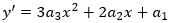
We now have enough information to state our four constraints in mathematical terms:

With a little algebraic manipulation, we can now solve for the four coefficients. This is the same result as given in Equations 2a through 2d:

The proofs for the end segments (equations 4 and 6) are similar, except that only three sample points are required, and the slope is only defined at the sample adjacent to the following (for the left-most case) or preceding (for the right-most case) segment.

Image Interpolation

Catmul-Rom spline interpolation can also be used to resample two-dimensional data sets, such as images.

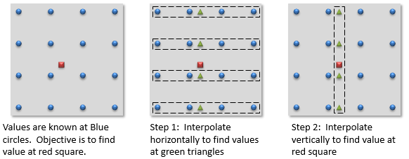
Figure 4: Interpolating 2D data sets, such as images

Suppose we know the pixel values at the blue dots (see Figure 4), and we want to know the value of the surface at the red square. The process requires two steps. In step one, we interpolate horizontally along the two rows above and two rows below the point in question. This gives us four new values (the green triangles) that are aligned vertically with the point we are trying to calculate. In step two, we use these four points to interpolate vertically to get the answer we want.

There are a couple of things worth noting about this method:

1. It turns out it doesn’t matter whether the initial set of four interpolations is done along the rows or along the columns of the image: the answer will be the same either way.
2. If the location you are trying to interpolate happens to align exactly with a row (or column), you don’t need to perform all five interpolations. It is sufficient to perform a single interpolation along that row (or column).

This is somewhat of a brute force method, requiring the calculation of five separate sets of cubic coefficients for each interpolated point. Fortunately, there is a more efficient implementation, which will be shown later.

Interpolating along a Two- or Three-Dimensional Path

Catmull-Rom spline interpolation can be used to fit a smooth curve between points on a 2D surface or through 3D space. Examples of when this may be required include:

• A computer graphics drawing application, where a user specifies a series of points on a drawing surface, and you need to draw a smooth line connecting those points.
• An Unmanned Air Vehicle (UAV) records GPS latitude, longitude and altitude at some sample rate, and you need to estimate the vehicle’s position between those points.

Figure 5a shows an example. There are six control points, each described by an (x,y) coordinate pair, and the goal is to interpolate a smooth spline curve that connects them.

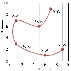
Figure 5a: Interpolation along a path defined by six control points.

To do the interpolation, the set of X coordinates and the set of Y coordinates are broken out into two separate lists, and the Catmul-Rom interpolation applied to each of them. For example, the X coordinates of points 1 through 6 in Figure 5a are (9, 6, 1, 1, 5, 7). This sequence is plotted as a function of the sample number in Figure 5b (green curve). Applying Catmull-Rom interpolation to this sequence yields the intermediate X coordinates for the curve. The same process is applied to obtain the Y coordinates (blue curve).

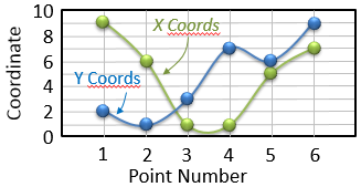
Figure 5b: Each dimension is interpolated separately.

This concept can be extended to an arbitrary number of dimensions.

It is worth noting that the derivation of Catmull-Rom interpolation implicitly assumes that the control points are equally spaced, a condition that is not necessarily met in a 2D graphics application. Although the technique is fairly forgiving in this regard, results can be poor if a series of control points includes a mixture of widely and closely spaced points. Some experimentation may be required.

Catmull-Rom Impulse Response: A More Efficient Implementation

The Catmull-Rom “impulse response” is the curve obtained by interpolating a signal consisting of a single sample of value 1.0, surrounded by samples of value 0.0, as illustrated in Figure 6.

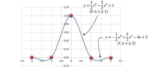
Figure 6: The Catmull-Rom Impulse Response (blue curve) is obtained by interpolating over a single unit-valued sample (red dots).

To obtain the equation for the impulse response between 0 and 1, we compute the Catmull-Rom coefficients of equations 2a through 2d using the values (0, 1, 0, 0) for y_a, y_b, y_c, and y_d, which gives us:

To obtain the equation for the impulse response between 1 and 2, we compute the Catmull-Rom coefficients of equation 2a through 2d using the values (1, 0, 0, 0) for y_a, y_b, y_c, and y_d, and then substitute (x-1) for x to shift the result, giving us:

The impulse response is symmetrical about 0, so we can define the negative portion of the curve by computing equations 11a and 11b using the absolute value of x.

Why is the impulse response important? Because convolving the impulse response with an arbitrary sampled signal gives us the interpolated signal. The process is illustrated in Figure 7:

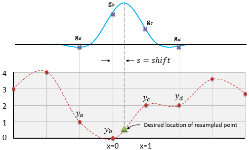
Figure 7: Interpolating an arbitrary sampled waveform by convolving it with the Catmull-Rom impulse response.

Suppose we know the values of the original waveform at points y_a, y_b, y_c and y_d. To calculate the interpolated value at some position x=s (the green triangle) requires the following steps:

1. Shift the convolution kernel (the Catmull-Rom impulse response, shown in blue) so that it is centered over the point to be interpolated.
2. Calculate the value of the Catmull-Rom impulse response at the four locations g_a, g_b, g_c and g_d, where they align with the four samples y_a, y_b, y_c and y_d.
3. Multiply the y values by the g values and sum them. That is, compute y(s) = g_ay_a + g_by_b + g_cy_c + g_dy_d. This is the interpolated value of the signal at x=s.

The four g values are sometimes called filter weights, and can be calculated as shown in equations 12a through 12d. The s term is the x coordinate of the point to be interpolated, relative to the nearest known sample to its left, and will always have a value between 0 and 1.

Given the four weights, the interpolated value at x=s is just:

As an example, let us suppose that we want to interpolate the signal shown in Figure 7 at a value of s=⅓ (that is, one-third of the distance between the two samples as shown). We evaluate equations (12a) through (12d), using a shift value of s=⅓, to obtain the four weights:

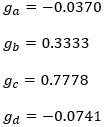
Then we multiply the four weights by the four known sample values (1, 0, 2, 2) and sum the result as in equation (13), to obtain:

So at x=⅓ the interpolated curve has a y value of 0.5185, which is the same answer we would have gotten from equations 1 and 2.

The amount of computation required using the convolution technique is not substantially different from the direct solution if you only need to interpolate a single point. But suppose you need to upsample a large waveform by some integer factor. The magic of the convolution approach is that you only need to compute the convolution weights (the g values) once. Thereafter, each resampling requires only four multiplications and four additions, whereas the direct solution from equations (1) and (2) requires a total of 12 multiplications and 12 additions. A little bookkeeping up front can therefore save a lot of computation time. This is even more true when resampling images, where the convolution approach requires only sixteen multiply-accumulate operations per resampled pixel.

Related Pages

• Interpolation Calculator. An interactive utility/demonstrator that calculates the coefficients to Equations 1, 3 and 5 for arbitrary sample values and displays the results graphicaly.

 

---

Comments and error reports may be sent to the following address. We may post comments of general interest. Be sure to identify the page you are commenting on.

.

---