Rotations in Three-Dimensions:
Euler Angles and Rotation Matrices
Part 1 - Main Paper
D. Rose - February, 2015
Abstract
This paper describes a commonly used set of Tait-Bryan Euler angles, shows how to convert from Euler angles to a rotation matrix and back, how to rotate objects in both the forward and reverse direction, and how to concatenate multiple rotations into a single rotation matrix.
The paper is divided into two parts. Part 1 provides a detailed explanation of the relevant assumptions, conventions and math. Part 2 provides a summary of the key equations, along with sample code in Java. (See the links at the top of the page.)
Anyone dealing with three dimensional rotations will need to be familiar with both Euler angles and rotation matrices. Euler angels are useful for describing 3D rotations in a way that is understandable to humans, and are therefore commonly seen in user interfaces. Rotation matrices, on the other hand, are the representation of choice when it comes to implementing efficient rotations in software.
Unfortunately, converting back and forth between Euler angles and rotation matrices is a perennial source of confusion. The reason is not that the math is particularly complicated. The reason is there are dozens of mutually exclusive ways to define Euler angles. Different authors are likely to use different conventions, often without clearly stating the underlying assumptions. This makes it difficult to combine equations and code from more than one source.
In this paper we will present one single (and very common) definition of Euler angles, and show how to use them.
Euler Angle Conventions
Euler angles are a set of three angles used to specify the orientation—or change in orientation—of an object in three dimensional space. Each of the three angles in a Euler angle triplet specifies an elemental rotation around one of the axes in a three-dimensional Cartesian coordinate system (see Figure 1). Unfortunately this is not a complete definition. To completely define a Euler angle system, one must choose from among the following possible permutations:
- Tait-Bryan vs. Classic: In the Tait-Bryan convention, each of the three angles in a Euler angle triplet defines the rotation around a different Cartesian axis. For example, the first angle may specify the rotation around the z axis, the second around the y axis, and the third around the x axis. For classic Euler angles, the three elemental rotations are performed around only two axes. For example, the first rotation may be around the z axis, the second around the y, and the third around the z axis again. Both systems are capable of representing all possible 3D rotations, and there is no inherent advantage of one over the other. However, most modern authors use the Tait-Bryan convention, and that is what we will use here. [Note: purists will claim that Tait-Bryan angles are not true Euler angles, but that view contravenes common usage.]
- Rotation order: When performing elemental rotations around each of the three axes, the order in which the rotations are executed matters. That is, performing elemental rotations around the axes in the order z, then y, then x will produce different results than performing the same rotations in any of the other five possible orders. For this paper, we will specify a rotation order of z, followed by y, followed by x.
- Intrinsic vs. Extrinsic rotations: In an intrinsic system, each of the elemental rotations is performed on the coordinate system as rotated by the previous operation(s). In an extrinsic system, each rotation is performed around the axes of the world coordinate system, which does not move. As an example, suppose the three angles of the Euler triplet specify rotations around the z, y, and x axes respectively, and in that order. The first elemental rotation around the z axis will be identical for both intrinsic and extrinsic conventions. However, for the intrinsic convention the second elemental rotation is performed around the y axis in its new position resulting from the first rotation, while in the extrinsic convention it is performed around the original (unrotated) y axis. Similarly, the final rotation around the x axis will be performed around the x axis as rotated by the first two operations in the intrinsic system, and around the original (unrotated) x axis in the extrinsic system. This paper will adhere to the intrinsic convention: i.e., the axes move with each rotation.
- Active vs. Passive rotations: Active rotation—also known as alibi rotation—is when the point is rotated relative to the coordinate system. Passive rotation—also known as alias rotation—is when the coordinate system rotates with respect to the point . The two conventions produce opposite rotations. This paper will adhere to the active convention.
- Coordinate system conventions: We will use a right-handed Cartesian coordinate system with right-handed rotations. In a right-handed coordinate system, if x̂, ŷ and ẑ are unit vectors along each of the three axis, then x̂ cross ŷ = ẑ. Right-handed rotation means rotations are positive clockwise when looking in the positive direction of any of the three axes.
To summarize, we will employ a Tait-Bryan Euler angle convention using active, intrinsic rotations around the axes in the order z-y-x. We will call the rotation angles yaw, pitch and roll respectively. This is a common convention, and most people find it the easiest to visualize. For example, the first two rotations (yaw and pitch) are identical to the azimuth and elevation angles used in directing artillery pieces and in surveying; to the pan and tilt angles used to specify the aiming direction of a camera; and to the longitude and latitude coordinates used in navigation. And of course the yaw-pitch-roll convention can be visualized as the change in orientation of an aircraft from the pilot’s perspective.
Figure 1 shows an example of this coordinate system centered on an aircraft. By convention, the x axis extends forward through the nose of the aircraft, the y axis points to the pilot’s right, and the z axis points down. The corresponding roll, pitch, and yaw rotation angles are positive in the directions indicated by the arrow circles.
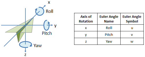
Figure 1: Euler Angle Axes, Names and Symbol Convention
Rotation order is: (1) Yaw, (2) Pitch and (3) Roll
In its initial position, the aircraft coordinate system and the world coordinate system are aligned with each other. If we want to rotate the aircraft, we perform the three elemental rotations as follows:
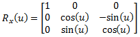
| Rotation around the x axis by roll angel (u): | x1 = x0 | (eq 1a) |
|
| y1 = y0cos(u) − z0sin(u) | (eq 1b) |
||
| z1 = y0sin(u) + z0cos(u) | (eq 1c) |
||
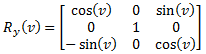
| Rotation around the y axis by pitch angle (v): | x2 = x1cos(v) + z1sin(v) | (eq 2a) |
|
| y2 = y1 | (eq 2b) |
||
| z2 = − x1sin(v) + z1cos(v) | (eq 2c) |
||
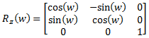
| Rotation around the z axis by yaw angle (w): | x3 = x2cos(w) − y2sin(w) | (eq 3a) |
|
| y3 = x2sin(w) + y2cos(w) | (eq 3b) |
||
| z3 = z2 | (eq 3c) |
where:
A point of clarification may be required concerning the order of operations. In the preceding paragraphs we stated that the elemental rotations would be conducted in the order yaw-pitch-roll; and yet equations 1, 2, and 3 are listed in the opposite order. This is not an error. Executing equations 1, 2 and 3 in the order shown will produce an intrinsic yaw-pitch-roll rotation, which is what we want. That is, to rotate a set of points by a yaw angle, followed by a pitch angle, followed by a roll angle using the intrinsic convention (where the axes move with each rotation), we must execute equations 1, 2, and 3 in the order shown. Executing the rotations in the opposite order (equations 3, then 2, then 1), results in an extrinsic yaw-pitch-roll rotation. In the general case, any intrinsic rotation can be converted to its extrinsic equivalent and vice-versa by reversing the order of elemental rotations.
Performing the three rotations separately as shown above is actually not a bad way to implement a 3D rotation. It requires only slightly more computation than the 3x3 matrix method (below), and makes it possible to experiment with one rotation at a time during debugging. It also makes it obvious how to change the order of rotations, should that be necessary. The primary drawback is that it makes it difficult to concatenate a series of rotations into a single rotation. For that you need to use rotation matrices.
To reverse a rotation (that is, to return a rotated point to its original coordinate in the reference frame), you simply reverse the order of the rotations, and also change the signs of the three rotation angles. So if the forward rotation is yaw(w), pitch(v), roll(u), then the inverse rotation is roll(-u), pitch(-v), yaw(-w).
Rotation Matrices
A rotation matrix is composed of nine numbers arranged in a 3x3 matrix like this:
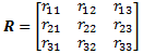
(eq 4)
Unlike Euler angles, rotation matrices require no assumptions about the order of elemental rotations. A given rotation can be described by many different sets of Euler angles depending on the order of elemental rotations, etc. But for any given rigid-body rotation, there is one and only one rotation matrix.
Rotating Points using a Rotation Matrix:
Given rotation matrix R, an arbitrary point can be rotated using the equation:

(eq 5)
In algebraic form, this expands to:
where:
Converting Euler Angles to a Rotation Matrix
The three elemental rotations presented in equations 1, 2, and 3 can be expressed in matrix form as:
| Rotation around the x axis by roll angle (u): | 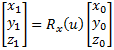 |
(eq 7a) |
|
| Rotation around the y axis by pitch angle (v): | 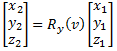 |
(eq 7b) |
|
| Rotation around the z axis by yaw angle (w)): | 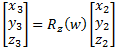 |
(eq 7c) |
(eq 8a)
(eq 8b)
(eq 8c)
Rather than performing each elemental rotation separately, we can combine the three rotation matrices of equations 8a, 8b and 8c into a single rotation matrix by multiplying them in the appropriate order.
The full rotation matrix for the elemental rotation order yaw-pitch-roll is (eq 9):
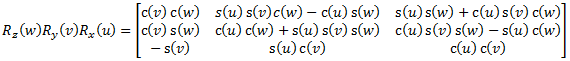
| (u, v, w) are the three Euler angles (roll, pitch, yaw), corresponding to rotations around the x, y and z axes | |
| c() and s() are shorthand for cosine and sine |
Converting a Rotation Matrix to Euler Angles
Given a rotation matrix, it is possible to convert back to Euler angles. Note that the equation will be different based on which set of Euler angles are desired (i.e., the order in which the Euler angle elemental rotations are intended to be executed). The Tait-Bryan Euler Angles corresponding to the order yaw-pitch-roll are:
| Yaw angle: | 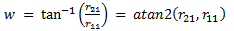 |
(eq 10a) |
|
| Pitch angle: | 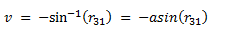 |
(eq 10b) |
|
| Roll angle: | 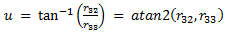 |
(eq 10c) |
The yaw and roll angles produced by equations 10a and 10c will always be in the range −π to +π (−180° to +180° ). The pitch angle will be between −π/2 and +π/2 (−90° to +90° ).
Gimbal Lock
Equations 10a through 10c are the general solution for extracting Euler angels from the rotation matrix. But consider what happens in the special case where the pitch angle v = +90° or −90°. Under both of these conditions, cos(v) = 0, and from equation 9 we can see that r11, r21, r32 and r33 must all equal zero. Since the atan2 function is not defined at (0,0), equations 10a and 10c are not valid when the pitch angle v = +/– 90°.This is the dreaded “gimbal lock.” It occurs because, at a pitch angle of + and – 90°, the yaw and roll axes of rotation are aligned with each other in the world coordinate system, and therefore produce the same effect. This means there is no unique solution: any orientation can be described using an infinite number of yaw and roll angle combinations. To handle the gimbal lock condition, we must detect when the pitch angle is +/- 90°. This can be accomplished directly (by finding the pitch angle v using equation 10b), or by testing r31.
If pitch angle v = −90°, then r31 will equal 1, and;
If pitch angle v = +90°, then r31 will equal −1, and;
In practice, we would set one of the angles to zero and solve for the other. For example, we could set the yaw angle (w) to zero and solve equations 11a and 11b for the roll angle (u).
It is worth noting that in the regions near the two gimbal lock points, the mapping from rotation-space to Euler angles is not continuous, meaning very small changes in orientation can result in discontinuous jumps in the corresponding Euler angles. For example, the Euler angles (0°,89°,0°) and (90°, 89°, 90°) represent orientations that are only about a degree apart, despite their very different numerical values. A good analogy is the way an aircraft’s longitude jumps discontinuously as it flies over the North or South Pole. This behavior causes problem when trying to interpolate between orientations, or find the average of multiple orientations (see below).
Note also that although Euler angles are susceptible to gimbal lock, rotation matrices are not. For every possible rotation there is one and only one rotation matrix. Also, for rotation matrices, the mapping is continuous. That is, small changes in rotation will always equate to small changes in the rotation matrix.
Inverse Rotations
In many practical applications it is necessary to know both the forward and the inverse rotation. Rotation matrices have the special property that the inverse equals the transpose (R−1 = RT). So if R is the forward rotation matrix, then the inverse matrix can be created simply by transposing the rows and columns of R:
| Forward rotation matrix: | 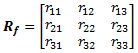 |
(eq 12) |
|
| Reverse rotation matrix: | 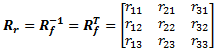 |
(eq 13) |
Combining Multiple Rotations
A series of rotations can be concatenated into a single rotation matrix by multiplying their rotation matrices together. For example, a rotation R1 followed by R2 can be combined into a single 3x3 rotation matrix by multiplying [R1][R2]. But once again, we need to be clear on our conventions.Consider that we have a list of points that define the 3D shape of an aircraft, in what we will call the normalized position—meaning the aircraft’s coordinate system is initially aligned with the world coordinate system. We want to give the aircraft a set of yaw, pitch and roll commands, causing it to rotate to a new orientation. We perform the following steps:
- Use the yaw, pitch and roll values to generate a rotation matrix (equation 9)
- Use the rotation matrix to rotate all the points that make up the aircraft (equation 6a, 6b and 6c)
Now the aircraft is rotated where we want it—so far so good.
Next we want to rotate the aircraft to a new orientation by giving it a second set of yaw, pitch and roll commands. These new commands are relative to the aircraft’s current orientation—that is, from the pilot’s current frame of reference. We perform the following steps:
- Use the second set of yaw, pitch and roll values to generate a second rotation matrix.
- Multiply the first matrix by the second matrix (in that order). This will produce a third 3x3 rotation matrix.
- Use the third matrix to rotate all the points from the original normalized point set.
If A is the current rotation matrix, B is the matrix describing the next relative orientation change, and C is the final rotation matrix to be applied to the normalized point set, then:
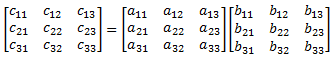
(eq 14)
where:
Caution: In matrix math, the order of multiplication matters. That is, multiplying matrix A times matrix B is not the same as multiplying B times A. The order of multiplication in equation 14 applies for intrinsic rotations, in which the axes move with each rotation. For extrinsic rotations (rotations around fixed world coordinates), the order of multiplication is reversed. This is a common source of confusion.
Interpolating Between Rotations, and Averaging Rotations
For some applications, it may be necessary to either interpolate between orientations, or to compute the average of a number of rotations.Interpolation is required is if, for example, we want to smoothly rotate a 3D object between two known orientations and need to generate the rotations for all the intermediate steps.
Averaging multiple rotations may be required when dealing with physical instrumentation such as Inertial Measurement Units (IMUs). For example, we may be implementing a virtual reality application in a smart phone, and need to determine what direction the phone is pointing. The phone will have several sensors such as accelerometers, gyroscopes, and/or a flux-gate compass that produce real-time orientation information at tens or hundreds of measurements per second—much faster than our application requires. However, we may find that each individual measurement is noisy, causing the image in our VR app to jump around. The solution is to smooth the data using a running average of the orientation information.
Unfortunately, it is not possible to compute either interpolations or averages using a Euler angle representation for rotations. The section on gimbal lock describes how the Euler angle representation jumps discontinuously in some parts of the rotation space. Trying to compute an average or interpolate across or near one of those critical regions will produce unreliable results.
It is possible (thought tedious) to interpolate between orientations using rotation matrices. The algorithm to do so is called “Spherical Linear Interpolation” (SLERP), a description of which may be found here (http://en.wikipedia.org/wiki/Slerp). It is also possible to compute the average of a set of rotation matrices, although once again the algorithm is tedious and somewhat ad hoc. The basic technique is:
- Sum the X column vectors, and normalize to unit length. (The X column vector is the three elements of the first column, treated as a vector). This produces the X column in the final average matrix.
- Sum the Y column vectors and normalize to unit length. This and the X vector define the X,Y plane.
- Compute the final average Y column vector by finding the unit vector that is perpendicular to the final X vector and in the X,Y plane.
- Compute the final average Z vector as the cross product of the final X and Y vectors.
- Make sure all three final column vectors in the average matrix are unit vectors and mutually orthogonal.
Although the above algorithms work, they are not recommended. If you need to do either interpolation or averaging of rotations, quaternions are the standard solution. Though somewhat intimidating at first, quaternions are a third technique for representing rotations (after Euler angles and rotation matrices), and provide an elegant and computationally efficient way to rotate points and concatenate, average, and interpolate rotations.
Rotation Matrix Properties
The following are properties of all rotation matrices:- The magnitude (sum of squares) of the elements in any row or column is 1. That is, each row and each column is a unit vector.
- The unit vectors in rows 1, 2 and 3 define the x, y and z axes of the rotated coordinate system in the original world space.
- The unit vectors in columns 1, 2, and 3 define the x, y, and z axes of the world coordinate system in the rotated coordinate space.
- The magnitude of all rows and all columns must be equal to 1.0
- The cross product of row 1 and row 2 must equal row 3
- The cross product of column 1 and column 2 must equal column 3
Comments and error reports may be sent to the following address. We may post comments of general interest. Be sure to identify the page you are commenting on.
 .
.
Correction Record:
- 21 Sep 2017: Equation 2, change v1 to z1. Thanks to David Roe for finding the error.
- 30 Mar 2016: Equation 10b, change asin(r31) to -asin(r31). Thanks to Adrian Schmutzler at the University of Bayreuth in Germany for finding the error.